
Abstract
We have recently developed a method to calculate thermodynamic properties of macroscopic systems by extrapolating properties of systems of molecular dimensions. Appropriate scaling laws for small systems were derived using the method for small systems thermodynamics of Hill, considering surface and nook energies in small systems of varying sizes. Given certain conditions, Hill's method provides the same systematic basis for small systems as conventional thermodynamics does for large systems. We show how the method can be used to compute thermodynamic data for the macroscopic limit from knowledge of fluctuations in the small system. The rapid and precise method offers an alternative to current more difficult computations of thermodynamic factors from Kirkwood–Buff integrals. When multiplied with computed Maxwell–Stefan diffusivities, agreement is found between computed predictions and experiments of the Fick diffusion coefficients for several binary systems. Diffusion coefficients were obtained by linking the Green–Kubo formulae to the Onsager coefficients. The formulae were used to improve/disprove empirical formulae for diffusion coefficients.
Export citation and abstract BibTeX RIS

Content from this work may be used under the terms of the Creative Commons Attribution 3.0 licence. Any further distribution of this work must maintain attribution to the author(s) and the title of the work, journal citation and DOI.
1. Introduction
Classical thermodynamics applies to systems on micrometer- or larger scales, as in the laboratory or in a chemical plant. Thermodynamic properties of nano-scale systems can be very far from the thermodynamic limit. It is well known that small systems are no longer extensive due to e.g. surface effects. Typical for a small system is that surface energies can be large. Even line and corner energies may contribute to the system energy.
Systems that no longer obey the extensivity we find on the large scale, can be understood as being small. Hill [1] proposed that the effect of such smallness can be handled by introducing an extra term in the classical thermodynamic equations. It is also necessary to specify the control variables, because unlike a large system, a small system has thermodynamic properties which depend on the environment. Using Hill's formalism one can derive equations for the effect of smallness on thermodynamic properties in an ensemble of interest. The small system that we have studied first [2–4] is controlled by the environment in such a way that it has constant chemical potential μ, volume V and temperature T. The thermodynamic limit is usually approached in computer simulations by using periodic boundary conditions. The effect of such boundary conditions has been well studied, see e.g. Landau et al [5] and Siepmann et al [6]. We can take advantage of properties of periodic boundary conditions to create a well-defined environment for the small system. The small system of interest is put inside a reservoir that has constant μ and T, and the effect of smallness is studied. At equilibrium, the number of particles and the energy of the small system will fluctuate. If the small system is sufficiently small compared to the size of the reservoir, however, it will be in the grand-canonical ensemble.
The important difference between the small and large scale system is illustrated in figure 1. Configurations illustrated in figure 1(a) are characteristic for systems with periodic boundary conditions, while the configurations in figure 1(b) are allowed for the small system. This setup creates surface energy for the small system. This presentation will focus on thermodynamic properties that follow from energy- and density fluctuations: the thermodynamic correction factor Γ, Kirkwood–Buff integrals and the molar enthalpy H.
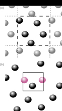
Figure 1. (a) Typical periodic boundary conditions as used in standard molecular dynamics simulations. (b) A small system controlled by a reservoir having constant chemical potential and temperature. The system is open and allows particles to enter at random. Due to lack of periodic boundary conditions as in (a) the system has an effective surface energy (adapted from Schnell et al [2]).
Download figure:
Standard image High-resolution imageThe thermodynamic correction factor is a measure of the deviation from ideal behaviour and can be used to convert Maxwell–Stefan diffusivities into Fick diffusivities. For an open single-component system, the thermodynamic correction factor follows from density fluctuations at a constant volume

where brackets denote an ensemble average, and N is the number of particles. The Kirkwood–Buff integral [7] provides derivatives of activity coefficients in mixtures from

where V is the volume, δij the Kroenecker delta and ci is the concentration of component i. The brackets denote averages in the grand-canonical ensemble. The molar enthalpy H can likewise be computed from energy and density fluctuations

where U is the potential energy of the system, and R is the universal gas constant. Using molecular dynamics simulations, we shall use these formulae to determine thermodynamic properties at different length scales. The characteristic length of the system, L = V1/d, is varied, see figure 2, where d is the system's dimension, here d = 3.

Figure 2. Systems of molecular size (with few particles) are positioned inside a large reservoir. The reservoir enclosing the boxes defines the variables which are controlled, and which are fluctuating. System properties can be computed from equations (1)–(3), and extrapolated to provide values for the macroscopic limit through equation (4) [3, 4].
Download figure:
Standard image High-resolution imageDepending on L, the thermodynamic properties differ from those of a large system, but in a predictable way. We find that the surface contributions scale linearly with 1/L, when surface energies are important [3, 7]:

We shall see how this scaling can be used in practice to determine thermodynamic properties of bulk systems from fluctuations in a system as small as a few particles. Line and nook energies will add terms of second and third order to these equations.
The method can also be used to determine surface thermodynamic data. The first step will be to determine the surface thickness of the adsorbed layer. This is done according to Gibbs [8]. The sampling area is varied, while the thickness of the surface is fixed. In this manner a two-dimensional thermodynamic surface system is created.
For more information regarding the details of the method in general, we refer to Schnell et al [4].
2. Application to diffusion
Diffusion is often a rate-limiting process in chemistry or biology, and reliable data of mixtures are scarce. This is so in particular for ternary systems, where no simulations have been done, and only a few experimental results are reported.
The generalized Fick equations for an n-component mixture can be written for the flux of each component i by
The total concentration is ct in mol m−3, xj is the mole fraction and Dij are Fick diffusivities. These equations are frequently the basis for reduction of experimental data. On the other hand, the Maxwell–Stefan (MS) equations are suitable for computations:

where the parenthesis gives the difference in the average velocities of components. Upright Dij are MS diffusivities. As both sets of equations must describe the same physical phenomena, the entropy production is invariant, and we obtain relations between variables. In vector notation we have [9]

where


The thermodynamic factors of the mixture are

where γi is the activity coefficient of component i, and the symbol Σ is used to indicate that the differentiation is carried out, while keeping constant the mole fractions of all other components, except the nth, so that the mole fractions sum to unity, see Liu et al [9] for further references. From knowledge of one set of diffusivities and corresponding thermodynamic factors, both as functions of concentration, one can therefore compute another set of diffusivities. This has been done using the method described in the previous section, and coefficients from experiments and simulations have been compared and found to agree remarkably well [9, 10], see below.
Knowledge of thermodynamic factors may in this manner facilitate the computational determination of Fick's diffusion coefficients which are difficult to measure.
3. Simulations
We tested first the performance of equations (1) and (2) at the small scale using molecular simulations for systems consisting of particles interacting either with a Lennard Jones (LJ) potential (truncated and shifted at 2.5σ, where σ is the molecular diameter) or a Weeks, Chander and Andersen (WCA)-potential (a shifted LJ potential with the attractive tail cut off, see Weeks et al [11]).
For convenience, the simulations were performed in reduced units, see Frenkel and Smit [12] for details. As the unit of length we use the particle diameter σ, and the unit of energy is the LJ-energy parameter,  . We simulated the large reservoir of particles in the micro-canonical ensemble, in which the small system of a varying size was embedded. The side of the small system (L = V1/d, where d is the system's dimension) was smaller than that of the half reservoir (Lt = Vt1/d), in order to ensure that the small system is unaffected by the periodic boundary conditions of the reservoir. With the WCA and LJ particles, the box side was Lt = 20.
The method was used to calculate the thermodynamic factor of mixtures, for which the diffusion coefficients were known experimentally. The Stefan–Maxwell diffusivities of the mixture components were computed along well defined schemes [9, 10]. The results of the calculations of the Stefan–Maxwell diffusivities were next combined with the results for the thermodynamic factor, using equations (5)–(10), to determine the Fick type diffusion coefficients. The outcome was compared with experimental results [9, 10].
4. Results and discussion
Results for the thermodynamic factor and for Kirkwood–Buff integrals are shown in figure 3. Both quantities are plotted as a function of 1/L. The dependence on 1/L is significant, meaning that the deviation from the thermodynamic limit is large for small systems. Similar results were obtained for the molar enthalpy (not shown).
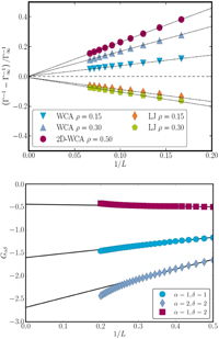
Figure 3. The thermodynamic factor (top) and the Kirkwood–Buff integral (bottom) plotted versus 1/L and extrapolated to provide their value in the thermodynamic limit.
Download figure:
Standard image High-resolution imageThe interesting fact is that the thermodynamic limit can be determined by extrapolation of small systems' properties. We have thus used the observed scaling property to predict properties of bulk systems by investigating properties of small systems! The lines in figure 3 are straight lines fitted to data for small systems with sizes L = 6–16 (0.06 < 1/L < 0.18). The value Lt = 20 prevented the small system from being affected by the periodic boundary conditions of the reservoir. We selected the value L = 6 as the smallest length of a small system to be investigated. With these values for L, one makes sure that we operate in the linear regime. The scaling law is the same for two- or three-dimensional systems (figure 3 top).
The method was also used to study surface adsorption, CO2 on a graphite surface [8]. We selected then a cylindrical volume element with thickness equal to the surface thickness, as measured by the CO2 layer adsorbed on the surface. The value of L was then the radius of the cylinder. We extended the size of the total surface in order to investigate a possible effect of Lt on the thermodynamic factor, see figure 4. The surface areas, Lt2, are labelled X1, X4 and X9, with X1 ∼ 50 × 50 Å2, X4 ∼ 100 × 100 Å2 and X9 ∼ 150 × 150 Å2. The figure shows results for 50 < N < 700, where N is the number of CO2 molecules in the system. The areas X4 and X9 give similar results, while X1 give results far from these. The area X4 has Lt equal to 20 (the length of CO2 ∼ 5 Å). This value corresponds well with the value referred to above. To find the thermodynamic factor, we therefore fitted results for 0.10 < 1/L < 0.40 to the linear equation (4) for N50 (for the other samples the region was slightly smaller), and made the extrapolation to the thermodynamic limit. From the thermodynamic factor, one can further obtain the chemical potential of the surface or the activity coefficient of the surface.
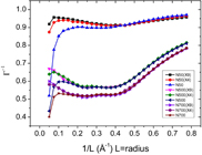
Figure 4. The inverse thermodynamic factor of CO2 on a graphite surface, as a function of the number N of CO2 particles in the system at reservoir area X1, X4 and X9 (see the text).
Download figure:
Standard image High-resolution imageThe sign of the slope in figure 3 is related to attractive and repulsive forces at the interface. It is not yet properly understood. The scaling is in sharp contrast to the finite-size scaling observed earlier for systems with periodic boundary conditions [6]. In equation (3), the constants C, D and B, are system-specific. Figure 3 reflects the linear term, except that nook- and corner effects are present for very small L, see [4]. Clearly, such effects can become important for very small system sizes.
The above results show that Monte Carlo simulations can be used to verify that Hill's approach to thermodynamics for small systems successfully describes the size dependence of thermodynamic properties of small systems embedded in a reservoir. We find a 1/L finite size scaling behaviour for the inverse thermodynamic correction factor Γ, the Kirkwood–Buff integral and the molar enthalpy H. The values of the slopes show that finite size effects are very important. The scaling behaviour can be used to connect thermodynamic properties obtained at different length scales. This gives a new way to determine thermodynamic properties of large and small systems.
The thermodynamic factor was found for binary mixtures and used to calculate Fick's diffusivities [9, 10], according to the description above, see figures 5 and 6.
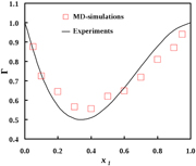
Figure 5. Thermodynamic factor for acetone in tetrachloromethane, as a function of mole fraction. Data are taken from Liu et al [9].
Download figure:
Standard image High-resolution image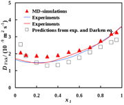
Figure 6. Fick's diffusivity of acetone in tetrachloromethane as a function of composition. Data are taken from Liu et al [9].
Download figure:
Standard image High-resolution image
The agreement between computed values (simulations) and experimental values is remarkable. Diffusion coefficients for binary and ternary systems can be obtained by linking the Green–Kubo formulae to the Onsager coefficients. The values can be further used to predict new and evaluate common formulae for diffusion coefficients of components in a mixture. The method was used favourably for ternary mixtures, where experimental data are few, and where computational data are non-existent up to this point.
5. Conclusion and perspective
A new scaling method [3, 4] was used to compute thermodynamic data for the macroscopic limit from knowledge of fluctuations in small systems. The rapid and precise method offers an alternative to more difficult computations of thermodynamic factors, say from Kirkwood–Buff integrals [7]. When multiplied with computed Maxwell–Stefan coefficients, agreement was found between computed predictions and experiments for several binary systems. Diffusion coefficients for binary and ternary systems can be obtained by linking the Green–Kubo formulae to the Onsager coefficients. The outcome formulae can improve/disprove empirical formulae for diffusion coefficients [9, 10].
The success of the procedure has interesting implications. In the first place, the procedure helps to define smallness, and precise thermodynamic relations on the nano-metre scale. In the second place, it helps define local equilibrium or validity of thermodynamic relations, and when this can be expected. Taking example from, say, simulations of zeolites, one can show that a volume element must be an appropriate fraction of a unit cell in order to speak of thermodynamic properties in a meaningful way.
Acknowledgments
SS, TJHV and SK acknowledge financial support from NWO-CW through an ECHO grant number 700.58.042 and computational resources through NCF grant numbers MP-213-11, MP-213-12 and MP-213-13.